Estimating Weight and CoG > Taking Uncertainty into Account
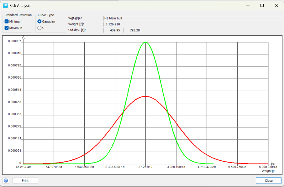
The Risk Analysis window shows how uncertainty affects the weight of a selected weight group or selected items. It plots a normal (Gaussian) distribution or its cumulative S-curve using the current weight and standard deviation. Use the curves to compare uncertainty assumptions and to estimate the probability of remaining below a chosen weight.
Open the window
In the main window, select the weight group to analyse, then choose Std.dev. > Risk Analysis. The window uses the selected group, rather than automatically using the total project weight. To analyse the total, select the relevant top weight group first.
In the Items window, select the required item rows, then choose View > Risk Curve, or Risk Curve from the right-click menu. Enable Item std.dev. field and select its code type under View > Options > Codes before using this item-based analysis. Check that the source standard-deviation values and their units are appropriate for the selected items.
The weight and standard-deviation fields are read-only. Prepare or calculate the uncertainty in the source data before opening the window; changing a curve option does not change the project weights or their stored uncertainty.
Values and controls
Wgt.grp.: Identifies the selected weight group. In item mode, the label changes to Wgt.grp. - Item no. and identifies the selected items.
Weight: The weight used as the centre of the normal distribution. For selected items, this is their combined weight. Read the unit displayed beside the field.
Std.dev.: The two standard-deviation values used for the Minimum and Maximum curves, in the displayed weight unit. These are measures of uncertainty, not minimum and maximum possible weights.
Minimum: Show the green curve based on the minimum standard deviation. For a sum of uncertain contributions, this assumes statistical independence: the combined standard deviation is the square root of the sum of the squared individual standard deviations.
Maximum: Show the red curve based on the maximum standard deviation. For a sum of uncertain contributions, this assumes fully positively dependent variations: the individual standard deviations are added directly. Both curves can be displayed together.
Gaussian: Show the bell-shaped probability-density curve. A larger standard deviation produces a broader, lower curve. The curve height at a single weight is a density, not the probability of that exact weight; probabilities correspond to areas under the curve.
S: Show the cumulative distribution. At a weight on the horizontal axis, the curve height estimates the probability that the weight is less than or equal to that value. The vertical scale runs from approximately 0 to 1; 0.90 represents 90%.
The window initially selects Minimum and Gaussian. Select at least one standard-deviation curve to display a result.
Read the graph
The horizontal axis shows weight, centred on the current weight, with markings relative to standard deviation (sigma). When Maximum is displayed, the horizontal range and sigma markings use the maximum standard deviation; otherwise they use the minimum. Changing the displayed curve can therefore change the axis scale.
To estimate the probability of staying below a weight limit, select S, find the limit on the horizontal axis and read the corresponding curve height. The probability of exceeding the limit is approximately 1 minus that value. With both curves shown, read each curve separately to compare the two dependency assumptions.
For example, with a weight of 1,000 t and a standard deviation of 50 t, a limit of 1,100 t is two standard deviations above the centre. Under the normal-distribution model, the S-curve gives approximately 0.977 (97.7%) below that limit and 2.3% above it. The window draws the curves numerically, so values read from the graph are approximate.
Minimum and Maximum describe different assumptions about how uncertainties combine. They are not confidence limits or guaranteed bounds. A useful interpretation depends on realistic source weights, standard deviations and dependency assumptions.
Print and copy
Print: Open a print preview of the current graph. The right-click menu inside the graph also provides Print. Output requires Estimate > Output permission.
Create Bitmap: Right-click inside the graph and select Create Bitmap to copy the displayed graph to the clipboard. Paste it into a document or an image editor. This command requires Estimate > Output permission.
Close: Close the window. Curve selections affect the displayed graph and do not edit the source data.
If no useful curve appears
Check that the selected weight group has a defined weight and a defined minimum standard deviation. The window reports missing values when it opens. A positive standard deviation is needed to draw a normal-distribution curve; zero uncertainty does not produce a normal bell curve in this window.
For item analysis, also check that rows are selected, item standard deviation is enabled, the correct code type is selected in Options > Codes, and the selected items contain usable uncertainty values. Close and reopen the window after correcting the source data.